Step 1 - Formatting

Before working with time series data, reformat the data to an appropriate format to work with. Formatting is everything when working with time series. It determines whether or not later testing will be successful or fail for strange reasons. The appropriate format to work with is very simple, the datetime information and the variable of interest. However, this means that any labels that go with this information need to be stripped prior to modeling. I would suggest storing the labels separately and iterating through the data and the labels concurrently when working with the model.

Step 2 - Scrubbing

When working with large amounts of data, sometimes it’s easy to miss little data idiosyncrasies that can really affect future modeling. For instance, in a project that I completed, I had all of the values for 349 out of 350 sets of time based data. For that last value, I was missing 78% of the time series data. I ended up backfilling the missing values with the first known value for that dataset.

Step 3 - Setting Up Model Parameters

Time Series data takes a little bit of work to navigate to a fit for an appropriate model. First, seasonal decomposition should be evaluated. I used seasonal_decompose from statsmodels.tsa.seasonal in my time series project. This decomposition shows information about the observed data, the general trend in the data, the seasonality, as well as the residuals. It is the included information about the residuals that I really appreciated about this particular decomposition function. If there is an identifiable pattern in the seasonality graph, determine the pattern for use in seasonal modeling. For my time series project there was a yearly season.

Additionally, the autocorrelation function (ACF) and the partial autocorrelation function (PACF) provide useful information for determining how a time series model should be set up. Ideally, both the ACF and PACF would show random walk data, examples of this can be see below in Figures 1 and 2. Random walk data is preferred for time series modeling because that means that there aren’t any underlying relationships present in the data that would interfere with the ability to make predictions. So, if you have random walk data, then it will be easy for your selected model to make accurate predictions.

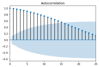Figure 1. ACF random walk

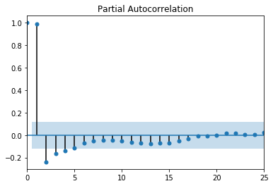Figure 2. PACF random walk

These plots, ACF and PACF, can help identify what values to use for the autoregressive (AR), differencing (I), and moving average (MA) parts of an ARIMA or SARIMA model. I used this reference when trying to interpret my ACF and PACF plots. Here, in Figure 2, there is something called lag happening at the PACF value of 1. Notice how the value flips from a positive to a negative value when moving from 1 to 2 on the x-axis. This likely means that the AR value best suited for this data is equivalent to the lag. So, for my p values in a time series model, I would evaluate 0 and 1. If this same pattern appears in the ACF plot, then consider adding an MA value equivalent to where the flip from positive to negative occurs. For this model, I would only evaluate a q value of zero, since the suggested pattern is missing. If the ACF plot is positive for a long time, as seen in Figure 1, then it is likely that a differencing value, or d, will be needed. The level of correlation remains high up to 15 lags, staying over 0.5 out of 1.0, as seen in Figure 1. So the d values that are most likely to work are 0, 1, or 2. If the correlation falls quickly, then I wouldn’t evaluate a d value of 2. Since I choose to evaluate differencing up to a value of 2, it would be wise to include a q value of 1 in the evaluation to compensate for over-differencing.

So, the model for my time series project needs to have a seasonal component, have p values 0 or 1, have d values of 0, 1, or 2, and have q values of 0 or 1.

Step 4 - Setting Up Metrics to Evaluate Model

In the ARIMA fucntion from statsmodels.tsa.arima_model there are two methods predict and forecast. The naming on these methods is misleading. The forecast method uses the generated model to generate predicted values for all dates present in the data passed in. In other words, the forecast method creates your predicted y values. The predict method is specifically for dates not used to create the model. The predict method is what could be used to validate the model.

To prepare for validating the model, data needs to be removed from what will be used to generate the model. So, a train-test split needs to be done. But this split is for time data, so it will look different. Depending on how much history you have in your dataset, you’ll need to chop off a portion at the end for this validation step.

Step 5 - Setting Up Predictions

Predictions are for times outside of the scope of your original data, and help inform decisions about the test case.

Step 6 - Modeling

At this point, you are ready to start modeling and figuring out the best solution for your data.